
American Election 2016 in California

Introduction
Welcome to my data exploration! Through this report, we will have an better insight about 2016 Presidential Campaign Finance 2016. The raw data is collected from website: http://fec.gov/disclosurep/pnational.do
The content of my report is organized by following sections:
-
Univariate Plots Section: multiple plots for individual variables.
-
Univariate Analysis: commment about the univariate finding.
-
Bivariate Plots Section: multiple plots for the relation between two variables
-
Bivariate Analysis: commment about the bivariate finding.
-
Multivariate Plots Section: multiple plots for the relation between three and more variables.
-
Multivariate Analysis: commment about the multivariate finding
-
Final Plots and Summary
-
Reflection
library(ggplot2)
library(ggthemes)
library(gridExtra)
library(dplyr)
library(plotly)
library(grid)
library(DT)
library(GGally)
library(psych)
Data structure
pf <- read.csv('P00000001-CA.csv')
pf$contbr_occupation[pf$contbr_occupation == "INFORMATION REQUESTED PER BEST EFFORTS"] <- "INFORMATION REQUESTED"
names(pf)
dim(pf)
str(pf)
pf_sample <- pf #using whole dataset
##  [1] "cmte_id"           "cand_id"           "cand_nm"
##  [4] "contbr_nm"         "contbr_city"       "contbr_st"
##  [7] "contbr_zip"        "contbr_employer"   "contbr_occupation"
## [10] "contb_receipt_amt" "contb_receipt_dt"  "receipt_desc"
## [13] "memo_cd"           "memo_text"         "form_tp"
## [16] "file_num"          "tran_id"           "election_tp"
## [19] "X"
## [1] 1040672 19
## 'data.frame':	1040672 obs. of  19 variables:
##  $ cmte_id          : Factor w/ 25 levels "C00458844","C00500587",..: 6 6 6 7 7 7 7 6 7 7 ...
##  $ cand_id          : Factor w/ 25 levels "P00003392","P20002671",..: 1 1 1 12 12 12 12 1 12 12 ...
##  $ cand_nm          : Factor w/ 25 levels "Bush, Jeb","Carson, Benjamin S.",..: 4 4 4 20 20 20 20 4 20 20 ...
##  $ contbr_nm        : Factor w/ 184410 levels " ALERIS, ANNAKIM",..: 6157 25050 55765 94017 95179 95179 95205 73475 95222 95242 ...
##  $ contbr_city      : Factor w/ 2077 levels "","-4086",".",..: 927 257 596 256 1476 1476 1965 891 2017 1349 ...
##  $ contbr_st        : Factor w/ 1 level "CA": 1 1 1 1 1 1 1 1 1 1 ...
##  $ contbr_zip       : Factor w/ 127038 levels "","00000","000090272",..: 101631 63495 47311 58650 15247 15247 40310 51776 54670 102865 ...
##  $ contbr_employer  : Factor w/ 54940 levels ""," APPLE INC.",..: 32438 32438 32438 3754 52045 52045 34655 32438 33559 42685 ...
##  $ contbr_occupation: Factor w/ 24164 levels ""," ATTORNEY",..: 18087 18087 18087 20209 15150 15150 16579 18087 14018 6202 ...
##  $ contb_receipt_amt: num  50 200 5 40 35 100 25 40 10 15 ...
##  $ contb_receipt_dt : Factor w/ 640 levels "01-APR-15","01-APR-16",..: 521 389 24 75 95 116 75 389 95 116 ...
##  $ receipt_desc     : Factor w/ 74 levels "","* EARMARKED CONTRIBUTION: SEE BELOW REATTRIBUTION/REFUND PENDING",..: 1 1 1 1 1 1 1 1 1 1 ...
##  $ memo_cd          : Factor w/ 2 levels "","X": 2 2 2 1 1 1 1 2 1 1 ...
##  $ memo_text        : Factor w/ 360 levels "","*","* $550 REFUNDED 6/16/16",..: 37 37 37 4 4 4 4 37 4 4 ...
##  $ form_tp          : Factor w/ 3 levels "SA17A","SA18",..: 2 2 2 1 1 1 1 2 1 1 ...
##  $ file_num         : int  1091718 1091718 1091718 1077404 1077404 1077404 1077404 1091718 1077404 1077404 ...
##  $ tran_id          : Factor w/ 1037291 levels "A000771210424405B8CF",..: 247724 247006 244388 773763 775207 777508 773225 247044 775203 778420 ...
##  $ election_tp      : Factor w/ 4 levels "","G2016","P2016",..: 3 3 3 3 3 3 3 3 3 3 ...
##  $ X                : logi  NA NA NA NA NA NA ...
In summary, this dataset has more than 1 million observations. This is quite a big data that can help me to know about the financial contribution of voters in California area during American Election 2016. Each observation contains 19 variables with multiple ordered factors. There is only 1 numeric variable, the amount of contribution or “contb_receipt_amt”.
1. Univariate Plots Section

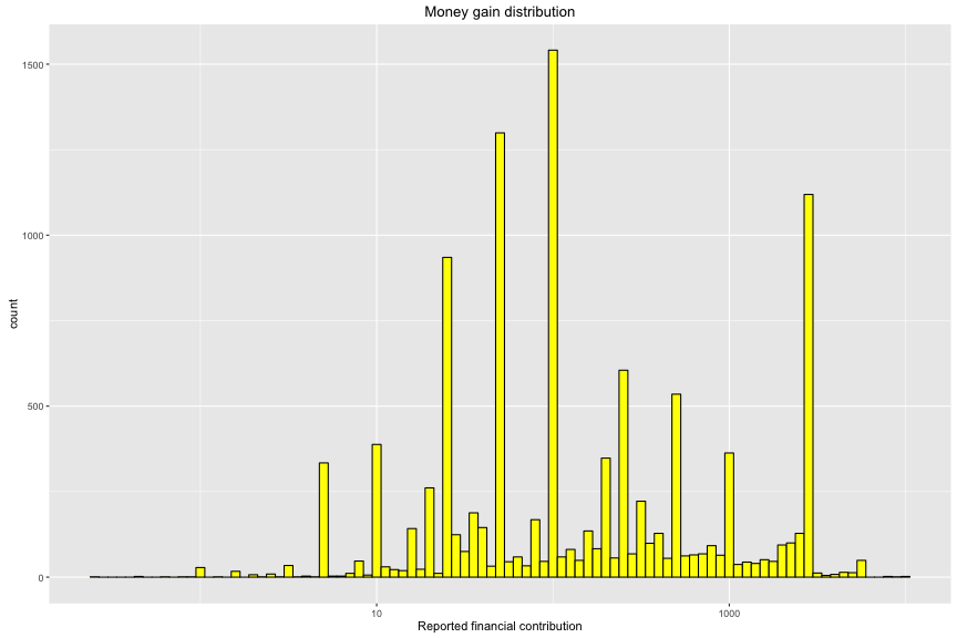
In the horizontal bar chart above, it is not uniform distribution. Number of contribution mainly go to Hilary Clinton or Bernard Sanders in CA. How is the distribution of money from contributors ?
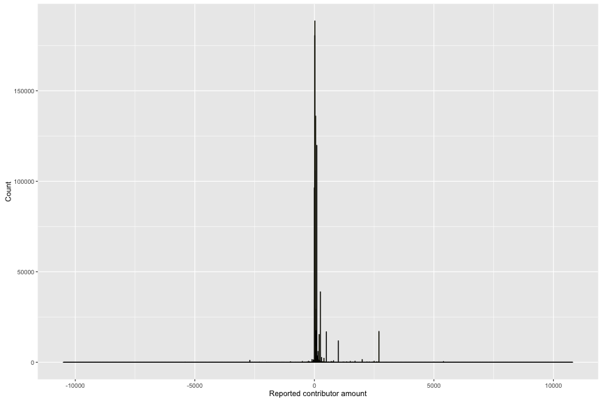
##     Min.  1st Qu.   Median     Mean  3rd Qu.     Max.
## -10500.0     15.0     27.0    123.1     87.5  10800.0
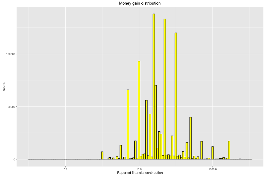
There is 75% of contribution that is from 15 usd to 87.5 usd to their candidates. In order to have better observation, I plotted the money contribution in range between 15 to 100 usd.
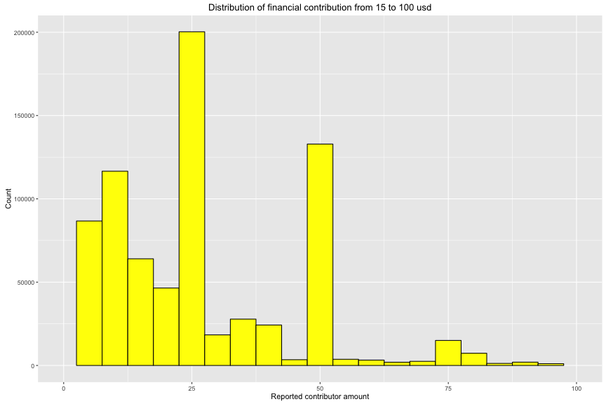
The peak is 25 usd/contribution. Through the summary of financial contribution, there are negative and positive money. The positive is the money to candidate fund and the negative is the money out of candidate fund. So, I seperate this variable into 2 subsets. By doing this, I will have better comparison to determine who win and lose in fund raising in this American Election 2016.
1.1. Positive Contribution
Let’s start with the positive subset. How is the contribution in this group ?

##     Min.  1st Qu.   Median     Mean  3rd Qu.     Max.
##     0.01    15.00    27.00   130.50    96.50 10800.00
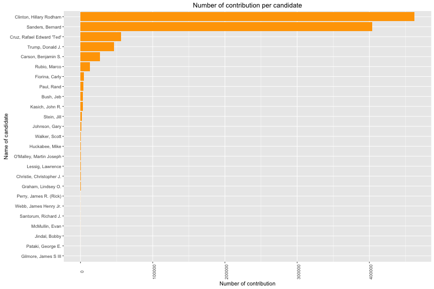
Top 5 candidates that get the largest contribution are Hilary Clinton, Bernard Sanders, Rafael “TED” Cruz, Donald Trump and Benjamin Carson respectively. However, Hilary Clinton and Bernard Sanders have large dominant positions. On the other hand, the money per contribution is very diversed and I have to use log10() function to display this distribution. The median is at 27 usd and 75% is from 15 to 130.5 usd. There are outliers with max at 10,800 usd.
1.2. Negative Contribution
##      Min.   1st Qu.    Median      Mean   3rd Qu.      Max.
## -10500.00   -500.00   -100.00   -565.50    -38.00     -0.24
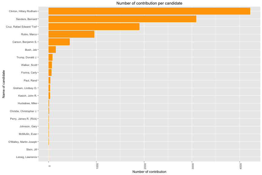
In contrast group, top 5 candidates that get largest number of negative contribution are Hilary Clinton, Bernard Sanders, Rafael “TED” Cruz, Marco Rubio and Benjamin Carson. Except Donald Trump, the top 4 candidates have highest postive contribution and also have highest negative contribution during this American Election in CA. In study of money per contribution, the median is - 100 usd and 75% is from -38 to -500 usd. The minimum is at -10,500 usd.
2. Univariate Analysis
What is the structure of your dataset?
There are 1,040,672 observations in the dataset with 19 variables. Except ‘contb_receipt_amt’, other features are ordered by factor variables with many levels.
## 'data.frame':	1040672 obs. of  19 variables:
##  $ cmte_id          : Factor w/ 25 levels "C00458844","C00500587",..: 6 6 6 7 7 7 7 6 7 7 ...
##  $ cand_id          : Factor w/ 25 levels "P00003392","P20002671",..: 1 1 1 12 12 12 12 1 12 12 ...
##  $ cand_nm          : Factor w/ 25 levels "Bush, Jeb","Carson, Benjamin S.",..: 4 4 4 20 20 20 20 4 20 20 ...
##  $ contbr_nm        : Factor w/ 184410 levels " ALERIS, ANNAKIM",..: 6157 25050 55765 94017 95179 95179 95205 73475 95222 95242 ...
##  $ contbr_city      : Factor w/ 2077 levels "","-4086",".",..: 927 257 596 256 1476 1476 1965 891 2017 1349 ...
##  $ contbr_st        : Factor w/ 1 level "CA": 1 1 1 1 1 1 1 1 1 1 ...
##  $ contbr_zip       : Factor w/ 127038 levels "","00000","000090272",..: 101631 63495 47311 58650 15247 15247 40310 51776 54670 102865 ...
##  $ contbr_employer  : Factor w/ 54940 levels ""," APPLE INC.",..: 32438 32438 32438 3754 52045 52045 34655 32438 33559 42685 ...
##  $ contbr_occupation: Factor w/ 24164 levels ""," ATTORNEY",..: 18087 18087 18087 20209 15150 15150 16579 18087 14018 6202 ...
##  $ contb_receipt_amt: num  50 200 5 40 35 100 25 40 10 15 ...
##  $ contb_receipt_dt : Factor w/ 640 levels "01-APR-15","01-APR-16",..: 521 389 24 75 95 116 75 389 95 116 ...
##  $ receipt_desc     : Factor w/ 74 levels "","* EARMARKED CONTRIBUTION: SEE BELOW REATTRIBUTION/REFUND PENDING",..: 1 1 1 1 1 1 1 1 1 1 ...
##  $ memo_cd          : Factor w/ 2 levels "","X": 2 2 2 1 1 1 1 2 1 1 ...
##  $ memo_text        : Factor w/ 360 levels "","*","* $550 REFUNDED 6/16/16",..: 37 37 37 4 4 4 4 37 4 4 ...
##  $ form_tp          : Factor w/ 3 levels "SA17A","SA18",..: 2 2 2 1 1 1 1 2 1 1 ...
##  $ file_num         : int  1091718 1091718 1091718 1077404 1077404 1077404 1077404 1091718 1077404 1077404 ...
##  $ tran_id          : Factor w/ 1037291 levels "A000771210424405B8CF",..: 247724 247006 244388 773763 775207 777508 773225 247044 775203 778420 ...
##  $ election_tp      : Factor w/ 4 levels "","G2016","P2016",..: 3 3 3 3 3 3 3 3 3 3 ...
##  $ X                : logi  NA NA NA NA NA NA ...
What is/are the main feature(s) of interest in your dataset ?
The main features in this dataset are contb_receipt_amt (CONTRIBUTION RECEIPT AMOUNT) and cand_nm (CANDIDATE NAME). I would like to know the financial support of each candidate in this AMERiCAN ELECTION 2016. My idea is that I can make a prediction about the financial contribution based on other features.
What other features in the dataset do you think will help support your investigation into your feature(s) of interest?
Name of city, occupation, candidate name likely contribute to the financial support.
Did you create any new variables from existing variables in the dataset?
Currently I do not make new variable for univariate analysis. I found that it is not necessary to find new variable while I only have 1 numeric variable (contb_receipt_amt) and the rest is catergory variables.
Of the features you investigated, were there any unusual distributions? Did you perform any operations on the data to tidy, adjust, or change the form of the data? If so, why did you do this?
I encountered with the positive and negative sign in financial contribution. Therefore, I created two dataset which contains only positive or negative support. It help me to have a good overview of money raising and losing for each candidate. I used log_10 tranformation to study about the financial support because its distribution is very skewed.
In positive support, contribution tends to give money at some fixed amount with a highest count around 50euro . So is negative support, the highest count is at 100 euro.
3. Bivariate Plots Section
Firstly, I extract information of some outliers from financial contribution.
3.1. Top contributors
3.1a. Positive contributor
##            cand_nm  contbr_nm contbr_zip
## 8950 Walker, Scott MUTH, RICK      90680
Scott Walker is the one who received the biggest money from contributor Rick Mut with 10,800.
##              cand_nm  contbr_nm contbr_zip contb_receipt_amt
## 8950   Walker, Scott MUTH, RICK      90680             10800
## 8951   Walker, Scott MUTH, RICK      90680             -5400
## 8952   Walker, Scott MUTH, RICK      90680             -2700
## 8953   Walker, Scott MUTH, RICK      90680              2700
## 988004 Walker, Scott MUTH, RICK      90680             -2700
##        contb_receipt_dt receipt_desc
## 8950          07-JUL-15
## 8951          07-JUL-15
## 8952          07-JUL-15
## 8953          07-JUL-15
## 988004        16-NOV-15       Refund
## [1] 2700
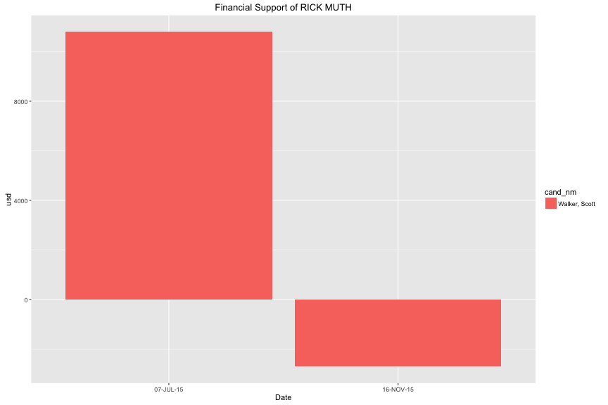
On 7-Jul, he contributed 10,800 usd. Later, he withrawed 8,100 usd then put in 2,700 usd again. After 4 month, he got back 2,700 usd. In final, he only contributed 2,700 usd to Scott Walker for this American Election.
3.1b. Negative contributor
##                 cand_nm       contbr_nm contbr_zip
## 583633 Sanders, Bernard BECK, NICOLETTE  941103415
The maximum money loss is 10,500 usd. Bernard Sanders is the one who lost largest money from contributor Nicolette Beck.
##                 cand_nm       contbr_nm contbr_zip contb_receipt_amt
## 10027  Sanders, Bernard BECK, NICOLETTE  941103415               500
## 14098  Sanders, Bernard BECK, NICOLETTE  941103415               500
## 38866  Sanders, Bernard BECK, NICOLETTE  941103415               500
## 61705  Sanders, Bernard BECK, NICOLETTE  941103415              5000
## 61706  Sanders, Bernard BECK, NICOLETTE  941103415               500
## 62974  Sanders, Bernard BECK, NICOLETTE  941103415              5000
## 106271 Sanders, Bernard BECK, NICOLETTE  941103415               500
## 130294 Sanders, Bernard BECK, NICOLETTE  941103415             -1800
## 131806 Sanders, Bernard BECK, NICOLETTE  941103415              -500
## 134337 Sanders, Bernard BECK, NICOLETTE  941103415              -250
## 158593 Sanders, Bernard BECK, NICOLETTE  941103415             -1000
## 206357 Sanders, Bernard BECK, NICOLETTE  941103415               500
## 352369 Sanders, Bernard BECK, NICOLETTE  941103415               500
## 361793 Sanders, Bernard BECK, NICOLETTE  941103415               250
## 379907 Sanders, Bernard BECK, NICOLETTE  941103415              1000
## 415093 Sanders, Bernard BECK, NICOLETTE  941103415              1000
## 437263 Sanders, Bernard BECK, NICOLETTE  941103415              4000
## 583633 Sanders, Bernard BECK, NICOLETTE  941103415            -10500
## 771202 Sanders, Bernard BECK, NICOLETTE  941103415              1000
## 783502 Sanders, Bernard BECK, NICOLETTE  941103415              1000
## 849788 Sanders, Bernard BECK, NICOLETTE  941103415               500
## 870541 Sanders, Bernard BECK, NICOLETTE  941103415               500
## 918846 Sanders, Bernard BECK, NICOLETTE  941103415             -4500
## 998664 Sanders, Bernard BECK, NICOLETTE  941103415             -2500
##        contb_receipt_dt
## 10027         01-AUG-15
## 14098         01-SEP-15
## 38866         01-FEB-16
## 61705         07-APR-16
## 61706         07-APR-16
## 62974         26-APR-16
## 106271        01-JUL-15
## 130294        30-NOV-15
## 131806        31-DEC-15
## 134337        21-MAR-16
## 158593        31-JUL-16
## 206357        01-DEC-15
## 352369        01-NOV-15
## 361793        28-JAN-16
## 379907        29-FEB-16
## 415093        09-NOV-15
## 437263        18-MAR-16
## 583633        25-JUN-16
## 771202        02-FEB-16
## 783502        08-JUN-16
## 849788        01-OCT-15
## 870541        01-MAR-16
## 918846        01-MAY-16
## 998664        04-APR-16
##                                                            receipt_desc
## 10027
## 14098
## 38866  * EARMARKED CONTRIBUTION: SEE BELOW REATTRIBUTION/REFUND PENDING
## 61705
## 61706
## 62974
## 106271
## 130294                                                           Refund
## 131806                                                           Refund
## 134337                                                           Refund
## 158593                                                           Refund
## 206357
## 352369
## 361793
## 379907 * EARMARKED CONTRIBUTION: SEE BELOW REATTRIBUTION/REFUND PENDING
## 415093
## 437263
## 583633                                                           Refund
## 771202 * EARMARKED CONTRIBUTION: SEE BELOW REATTRIBUTION/REFUND PENDING
## 783502
## 849788
## 870541
## 918846                                                           Refund
## 998664                                                           Refund
## [1] 1700
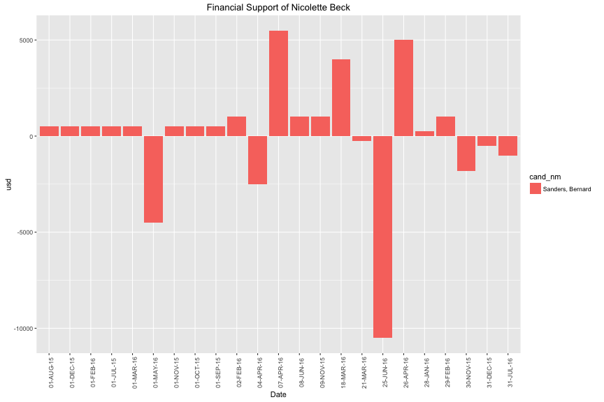
Morover, the interesting point is that this contributor did transaction to Bernard Sanders in multiple times. At last, the money for Bernard Sanders from this contributor is 1,700 usd in total.
3.2. Financial Support vs other features of interest
Since I have 18 features ordered by factor variables and the number of factors in my interested variables are large. It would be wise to make additional selections for each variables.
## Factor w/ 25 levels "Bush, Jeb","Carson, Benjamin S.",..: 4 4 4 20 20 20 20 4 20 20 ...
## Factor w/ 2077 levels "","-4086",".",..: 927 257 596 256 1476 1476 1965 891 2017 1349 ...
## Factor w/ 24164 levels ""," ATTORNEY",..: 18087 18087 18087 20209 15150 15150 16579 18087 14018 6202 ...
## Source: local data frame [5 x 1]
##
##                     cand_nm
##                      <fctr>
## 1              Rubio, Marco
## 2 Cruz, Rafael Edward 'Ted'
## 3   Clinton, Hillary Rodham
## 4          Sanders, Bernard
## 5       Carson, Benjamin S.
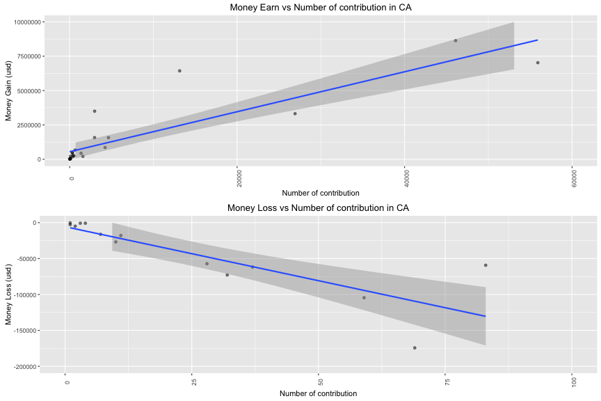
In money gain:
##
## Call:
## lm(formula = Money ~ Count, data = by_cand_nm_p)
##
## Coefficients:
## (Intercept)        Count
##      596730          116
##
## 	Pearson's product-moment correlation
##
## data:  by_cand_nm_p$Money and by_cand_nm_p$Count
## t = 9.067, df = 23, p-value = 0.000000004692
## alternative hypothesis: true correlation is not equal to 0
## 95 percent confidence interval:
##  0.7512196 0.9479820
## sample estimates:
##       cor
## 0.8839635
##     Min.  1st Qu.   Median     Mean  3rd Qu.     Max.
##     8100   188800   482900  5373000  3318000 77270000
In money loss:
##
## Call:
## lm(formula = Money ~ Count, data = by_cand_nm_m)
##
## Coefficients:
## (Intercept)        Count
##   -125217.1       -339.9
##
## 	Pearson's product-moment correlation
##
## data:  by_cand_nm_m$Money and by_cand_nm_m$Count
## t = -5.31, df = 18, p-value = 0.0000477
## alternative hypothesis: true correlation is not equal to 0
## 95 percent confidence interval:
##  -0.9093826 -0.5177217
## sample estimates:
##       cor
## -0.781255
##     Min.  1st Qu.   Median     Mean  3rd Qu.     Max.
## -1592000  -247900   -60540  -313900   -13390     -300
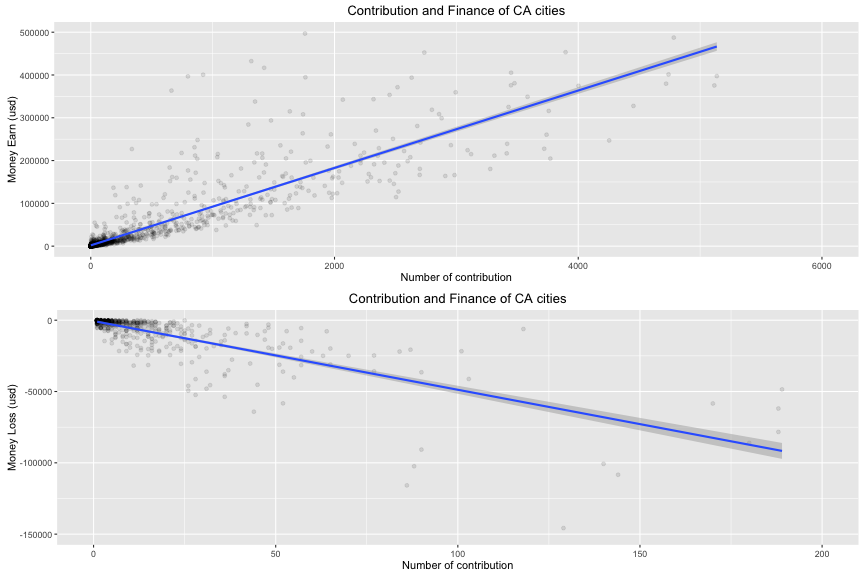
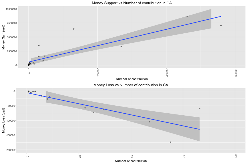
As number of contributions increases, the amount of money increases. This phenomenan happens in both money gain and money loss. The relationship between contributions and money apprers to be linear.
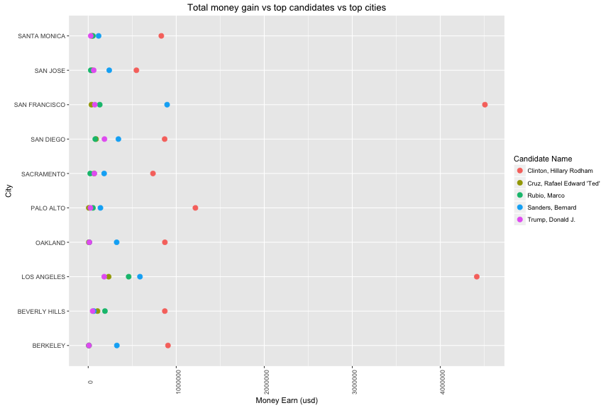
Next, I observe the financial contribution and amount of money related to cities in LA.
In money gain:
##
## Call:
## lm(formula = Money ~ Count, data = by_cities_p)
##
## Coefficients:
## (Intercept)        Count
##    -16410.7        163.5
##
## 	Pearson's product-moment correlation
##
## data:  by_cities_p$Money and by_cities_p$Count
## t = 142.59, df = 2069, p-value < 0.00000000000000022
## alternative hypothesis: true correlation is not equal to 0
## 95 percent confidence interval:
##  0.9485547 0.9565243
## sample estimates:
##      cor
## 0.952703
##     Min.  1st Qu.   Median     Mean  3rd Qu.     Max.
##        2      230     1827    64870    16020 14880000
In money loss:
##
## Call:
## lm(formula = Money ~ Count, data = by_cities_m)
##
## Coefficients:
## (Intercept)        Count
##      1287.6       -637.3
##
## 	Pearson's product-moment correlation
##
## data:  by_cities_m$Money and by_cities_m$Count
## t = -57.418, df = 617, p-value < 0.00000000000000022
## alternative hypothesis: true correlation is not equal to 0
## 95 percent confidence interval:
##  -0.9293844 -0.9044072
## sample estimates:
##       cor
## -0.917799
##    Min. 1st Qu.  Median    Mean 3rd Qu.    Max.
## -699300   -7386   -1926  -10140    -450     -10
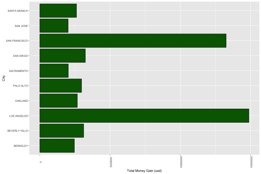
I have a high correlation between number of contribution and money gain per city. The city which has high number of contribution likely has high financial support for the election. Moreover, 75% of cities have contributed from 230 usd to 1827 usd (the median = 1827, the max = 14 millions). On the other side, money loss is larger when the number of contribution increases. There is 75% of cities which have money loss from 7,000 usd to 10,000 usd (the median = 1926 usd and the max = ~700,000 usd)
In money gain:
##
## Call:
## lm(formula = Money ~ Count, data = by_occupation_p)
##
## Coefficients:
## (Intercept)        Count
##     1326.99        99.34
##
## 	Pearson's product-moment correlation
##
## data:  by_occupation_p$Money and by_occupation_p$Count
## t = 382.79, df = 24160, p-value < 0.00000000000000022
## alternative hypothesis: true correlation is not equal to 0
## 95 percent confidence interval:
##  0.9247222 0.9282923
## sample estimates:
##       cor
## 0.9265281
##     Min.  1st Qu.   Median     Mean  3rd Qu.     Max.
##        1      125      315     5560     1000 20610000
In money loss:
##
## Call:
## lm(formula = Money ~ Count, data = by_occupation_m)
##
## Coefficients:
## (Intercept)        Count
##     -2321.5       -472.6
##
## 	Pearson's product-moment correlation
##
## data:  by_occupation_m$Money and by_occupation_m$Count
## t = -339.42, df = 442, p-value < 0.00000000000000022
## alternative hypothesis: true correlation is not equal to 0
## 95 percent confidence interval:
##  -0.9984126 -0.9976950
## sample estimates:
##        cor
## -0.9980872
##     Min.  1st Qu.   Median     Mean  3rd Qu.     Max.
## -3708000    -2954    -1290   -14140     -200       -1
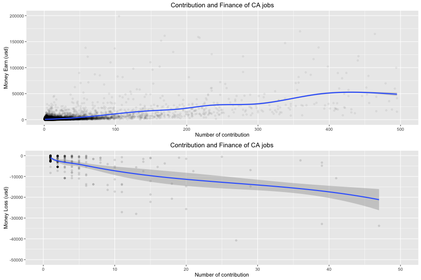
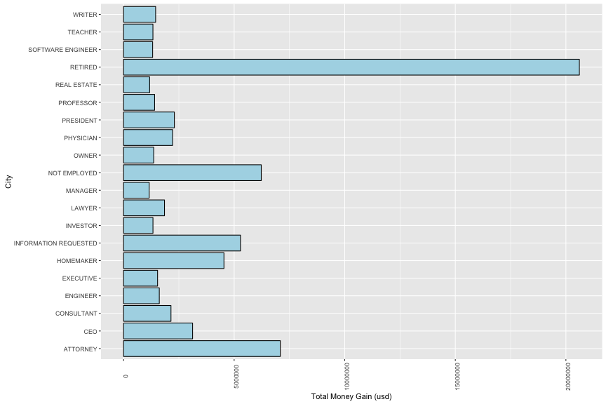
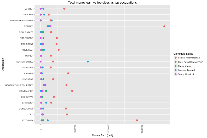
It states that the amount of money highly related to the number of contribution per job (the median = 315 usd and the max = 20 millions usd ). This pattern appears in the negative support too (the median = 1290 usd and the max = 3.7 millions).
For extra bivariate plots, I explored the financial support of contributors in two subsets that have those features:
-
In top 5 candidate.
-
In top 10 cities.
-
In top 20 occupation.
3.3. Extra exploration: Positive Contribution
I started exploring subdata with positive contribution since it is the most important one.
## [1] 125565 4
## Error in file(con, "rb"): cannot open the connection
My data have 123,077 observatations with 4 selective variables. I want to look closer at box plots involving financial support and other variables. By limiting the y axis, the boxplot observation is better. Let start with candidate:
3.3a Financial Support vs Candidate Name
## target_pf$candidate_name: Clinton, Hillary Rodham
##    Min. 1st Qu.  Median    Mean 3rd Qu.    Max.
##    0.04   20.00   50.00  234.20  100.00 5400.00
## --------------------------------------------------------
## target_pf$candidate_name: Cruz, Rafael Edward 'Ted'
##    Min. 1st Qu.  Median    Mean 3rd Qu.    Max.
##     1.0    25.0    50.0   220.2   100.0 10800.0
## --------------------------------------------------------
## target_pf$candidate_name: Rubio, Marco
##    Min. 1st Qu.  Median    Mean 3rd Qu.    Max.
##     3.0    40.0   100.0   742.9  1000.0  5400.0
## --------------------------------------------------------
## target_pf$candidate_name: Sanders, Bernard
##     Min.  1st Qu.   Median     Mean  3rd Qu.     Max.
##     1.00    15.00    27.00    63.48    50.00 10000.00
## --------------------------------------------------------
## target_pf$candidate_name: Trump, Donald J.
##    Min. 1st Qu.  Median    Mean 3rd Qu.    Max.
##     0.8    28.0    50.0   211.7   160.0  5400.0
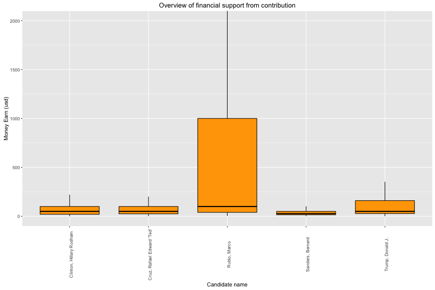
All of 5 candidates have non-normal distribution of financial supports. Therefore, using median value is better choice than using mean value. Marco Rubio has biggest median of positive support (median = 100) and Bernard Sanders has smallest one (median = 27).
3.3b. Financial Support vs Location
## target_pf$city: BERKELEY
##     Min.  1st Qu.   Median     Mean  3rd Qu.     Max.
##    1.000   20.000   50.000  140.097  100.000 2700.000
## --------------------------------------------------------
## target_pf$city: BEVERLY HILLS
##      Min.   1st Qu.    Median      Mean   3rd Qu.      Max.
##     0.640    27.000   100.000   566.626   500.000 10800.000
## --------------------------------------------------------
## target_pf$city: LOS ANGELES
##      Min.   1st Qu.    Median      Mean   3rd Qu.      Max.
##     0.160    18.550    35.000   204.181   100.000 10800.000
## --------------------------------------------------------
## target_pf$city: OAKLAND
##      Min.   1st Qu.    Median      Mean   3rd Qu.      Max.
##    0.4100   15.0000   35.0000  110.1563  100.0000 2700.0000
## --------------------------------------------------------
## target_pf$city: PALO ALTO
##     Min.  1st Qu.   Median     Mean  3rd Qu.     Max.
##    0.040   25.000   50.000  306.196  150.000 5000.000
## --------------------------------------------------------
## target_pf$city: SACRAMENTO
##     Min.  1st Qu.   Median     Mean  3rd Qu.     Max.
##    1.000   15.000   27.000  113.428  100.000 5400.000
## --------------------------------------------------------
## target_pf$city: SAN DIEGO
##     Min.  1st Qu.   Median     Mean  3rd Qu.     Max.
##    0.800   15.000   28.000   95.631   80.000 5400.000
## --------------------------------------------------------
## target_pf$city: SAN FRANCISCO
##     Min.  1st Qu.   Median     Mean  3rd Qu.     Max.
##     0.25    25.00    50.00   203.29   100.00 10000.00
## --------------------------------------------------------
## target_pf$city: SAN JOSE
##     Min.  1st Qu.   Median     Mean  3rd Qu.     Max.
##    1.000   10.000   27.000   82.061   50.000 5400.000
## --------------------------------------------------------
## target_pf$city: SANTA MONICA
##     Min.  1st Qu.   Median     Mean  3rd Qu.     Max.
##    0.650   19.000   38.000  220.999  100.000 5400.000
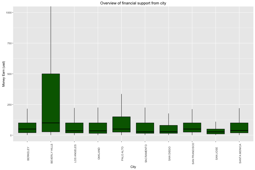
Most contributions (75%) from top 10 cities are varied from 18 to 100 usd. Beverly Hills is the city which has hightest median of contribution. Sacramento and San Jose are the least one.
3.3c Financial Support vs Occupation
## target_pf$occupation: ATTORNEY
##     Min.  1st Qu.   Median     Mean  3rd Qu.     Max.
##    0.160   25.000   50.000  292.647  200.000 5400.000
## --------------------------------------------------------
## target_pf$occupation: CEO
##      Min.   1st Qu.    Median      Mean   3rd Qu.      Max.
##     1.000    28.000   100.000   624.535   500.000 10800.000
## --------------------------------------------------------
## target_pf$occupation: CONSULTANT
##     Min.  1st Qu.   Median     Mean  3rd Qu.     Max.
##    0.330   19.000   50.000  224.553  100.000 5400.000
## --------------------------------------------------------
## target_pf$occupation: ENGINEER
##    Min. 1st Qu.  Median    Mean 3rd Qu.    Max.
##    1.00   25.00   50.00  131.97  100.00 4000.00
## --------------------------------------------------------
## target_pf$occupation: EXECUTIVE
##    Min. 1st Qu.  Median    Mean 3rd Qu.    Max.
##       1      38     100     472     250    5400
## --------------------------------------------------------
## target_pf$occupation: HOMEMAKER
##     Min.  1st Qu.   Median     Mean  3rd Qu.     Max.
##    1.000   19.000   50.000  432.113  250.000 5400.000
## --------------------------------------------------------
## target_pf$occupation: INFORMATION REQUESTED
##      Min.   1st Qu.    Median      Mean   3rd Qu.      Max.
##     0.800    40.000   100.000   297.547   250.000 10800.000
## --------------------------------------------------------
## target_pf$occupation: INVESTOR
##     Min.  1st Qu.   Median     Mean  3rd Qu.     Max.
##    1.000   50.000  200.000  879.424 2500.000 5400.000
## --------------------------------------------------------
## target_pf$occupation: LAWYER
##     Min.  1st Qu.   Median     Mean  3rd Qu.     Max.
##    1.000   25.000   67.640  315.084  250.000 5000.000
## --------------------------------------------------------
## target_pf$occupation: MANAGER
##      Min.   1st Qu.    Median      Mean   3rd Qu.      Max.
##    0.0400   15.0000   27.0000  152.7112  100.0000 2700.0000
## --------------------------------------------------------
## target_pf$occupation: NOT EMPLOYED
##     Min.  1st Qu.   Median     Mean  3rd Qu.     Max.
##    1.000   15.000   27.000   65.533   50.000 5000.000
## --------------------------------------------------------
## target_pf$occupation: OWNER
##     Min.  1st Qu.   Median     Mean  3rd Qu.     Max.
##    1.000   25.000   75.000  404.904  250.000 5400.000
## --------------------------------------------------------
## target_pf$occupation: PHYSICIAN
##    Min. 1st Qu.  Median    Mean 3rd Qu.    Max.
##    0.41   25.00   75.00  194.65  125.00 5400.00
## --------------------------------------------------------
## target_pf$occupation: PRESIDENT
##     Min.  1st Qu.   Median     Mean  3rd Qu.     Max.
##    1.000   25.000  100.000  582.351  500.000 5400.000
## --------------------------------------------------------
## target_pf$occupation: PROFESSOR
##      Min.   1st Qu.    Median      Mean   3rd Qu.      Max.
##    1.0000   21.0000   38.0000  140.5725  100.0000 2700.0000
## --------------------------------------------------------
## target_pf$occupation: REAL ESTATE
##     Min.  1st Qu.   Median     Mean  3rd Qu.     Max.
##    0.690   25.000   64.000  495.937  250.000 5400.000
## --------------------------------------------------------
## target_pf$occupation: RETIRED
##     Min.  1st Qu.   Median     Mean  3rd Qu.     Max.
##    0.390   16.550   28.445  126.453  100.000 8800.000
## --------------------------------------------------------
## target_pf$occupation: SOFTWARE ENGINEER
##     Min.  1st Qu.   Median     Mean  3rd Qu.     Max.
##    1.000   19.000   38.225  104.432  100.000 4000.000
## --------------------------------------------------------
## target_pf$occupation: TEACHER
##      Min.   1st Qu.    Median      Mean   3rd Qu.      Max.
##    1.0000   10.0000   25.0000   61.7222   50.0000 2700.0000
## --------------------------------------------------------
## target_pf$occupation: WRITER
##      Min.   1st Qu.    Median      Mean   3rd Qu.      Max.
##    0.6400   15.0000   31.5000  190.8828  100.0000 3000.0000
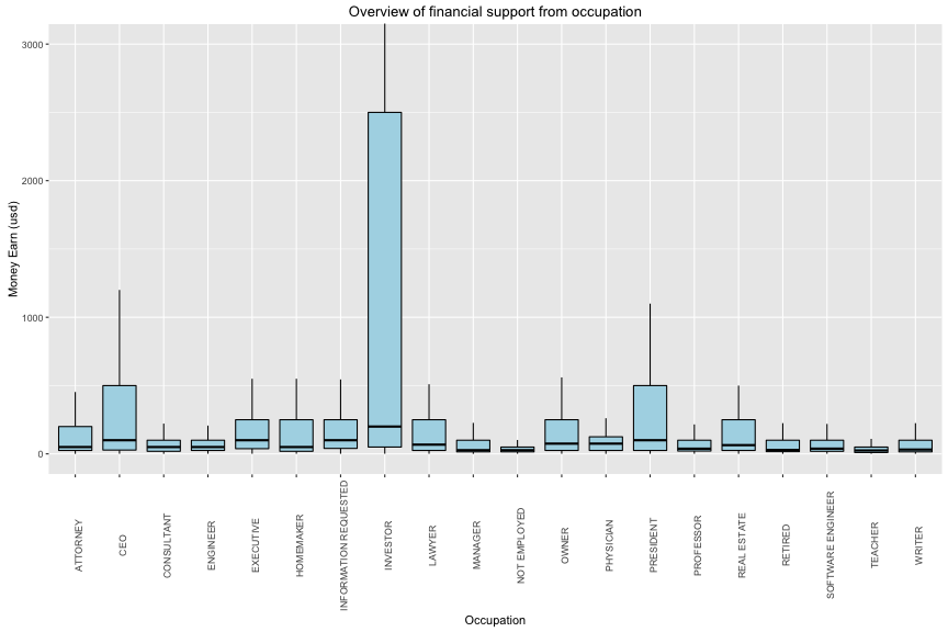
In next catergory, the most contribution to American Election is from retire people with have more than 20 millions usd (median = 28.445 and the = 8800)
3.3d. Cross Correlation between features of interest
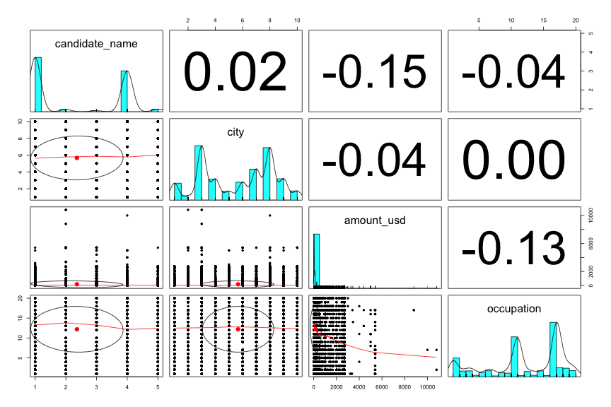
In general, the correlation between my interested variables are very low. The contribution is very diversed in city, occupation, employer and money to candidates.
###3.4. Extra exploration: Negative contribution
## [1] 2506 4
## Error in file(con, "rb"): cannot open the connection
3.4a. Financial Support vs Candidate Name
There are only 330 observations that satify my criteria.
## target_pf$candidate_name: Clinton, Hillary Rodham
##    Min. 1st Qu.  Median    Mean 3rd Qu.    Max.
##    0.04   20.00   50.00  234.20  100.00 5400.00
## --------------------------------------------------------
## target_pf$candidate_name: Cruz, Rafael Edward 'Ted'
##    Min. 1st Qu.  Median    Mean 3rd Qu.    Max.
##     1.0    25.0    50.0   220.2   100.0 10800.0
## --------------------------------------------------------
## target_pf$candidate_name: Rubio, Marco
##    Min. 1st Qu.  Median    Mean 3rd Qu.    Max.
##     3.0    40.0   100.0   742.9  1000.0  5400.0
## --------------------------------------------------------
## target_pf$candidate_name: Sanders, Bernard
##     Min.  1st Qu.   Median     Mean  3rd Qu.     Max.
##     1.00    15.00    27.00    63.48    50.00 10000.00
## --------------------------------------------------------
## target_pf$candidate_name: Trump, Donald J.
##    Min. 1st Qu.  Median    Mean 3rd Qu.    Max.
##     0.8    28.0    50.0   211.7   160.0  5400.0
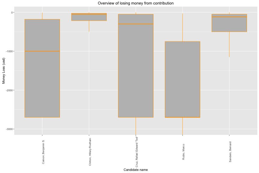
Rubio has the largest range of losing money -500 to -2700 usd. Donal Trump has the shortest range of losing money.
3.4b. Financial Support vs Location
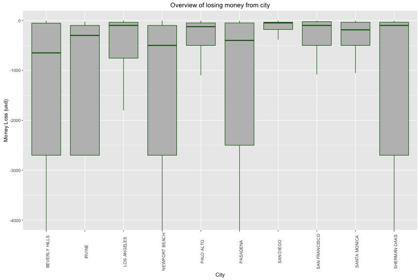
## target_pf_nega$city: BEVERLY HILLS
##      Min.   1st Qu.    Median      Mean   3rd Qu.      Max.
## -5400.000 -2700.000  -650.000 -1300.842   -54.430    -2.000
## --------------------------------------------------------
## target_pf_nega$city: IRVINE
##      Min.   1st Qu.    Median      Mean   3rd Qu.      Max.
## -2700.000 -2700.000  -300.000 -1131.091  -100.000   -25.000
## --------------------------------------------------------
## target_pf_nega$city: LOS ANGELES
##      Min.   1st Qu.    Median      Mean   3rd Qu.      Max.
## -5400.000  -755.250  -100.000  -657.504   -38.000    -0.240
## --------------------------------------------------------
## target_pf_nega$city: NEWPORT BEACH
##      Min.   1st Qu.    Median      Mean   3rd Qu.      Max.
## -4600.000 -2700.000  -500.000 -1214.513  -100.000    -1.000
## --------------------------------------------------------
## target_pf_nega$city: PALO ALTO
##       Min.    1st Qu.     Median       Mean    3rd Qu.       Max.
## -3000.0000  -500.0000  -125.0000  -586.4236   -50.0000    -5.0000
## --------------------------------------------------------
## target_pf_nega$city: PASADENA
##      Min.   1st Qu.    Median      Mean   3rd Qu.      Max.
## -5403.070 -2500.000  -400.000  -997.743   -50.000    -5.000
## --------------------------------------------------------
## target_pf_nega$city: SAN DIEGO
##      Min.   1st Qu.    Median      Mean   3rd Qu.      Max.
## -5400.000  -180.993   -50.000  -275.923   -35.750    -0.440
## --------------------------------------------------------
## target_pf_nega$city: SAN FRANCISCO
##       Min.    1st Qu.     Median       Mean    3rd Qu.       Max.
## -10500.000   -500.000   -100.000   -508.303    -25.000     -0.440
## --------------------------------------------------------
## target_pf_nega$city: SANTA MONICA
##      Min.   1st Qu.    Median      Mean   3rd Qu.      Max.
## -5400.000  -500.000  -188.075  -661.821   -38.000    -5.000
## --------------------------------------------------------
## target_pf_nega$city: SHERMAN OAKS
##      Min.   1st Qu.    Median      Mean   3rd Qu.      Max.
## -4315.000 -2700.000  -100.000 -1098.661   -36.000    -5.000
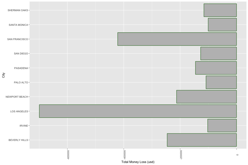
The city that have most money loss is Los Angeles with 700,000 usd (the median = -750, the max = -5,400)
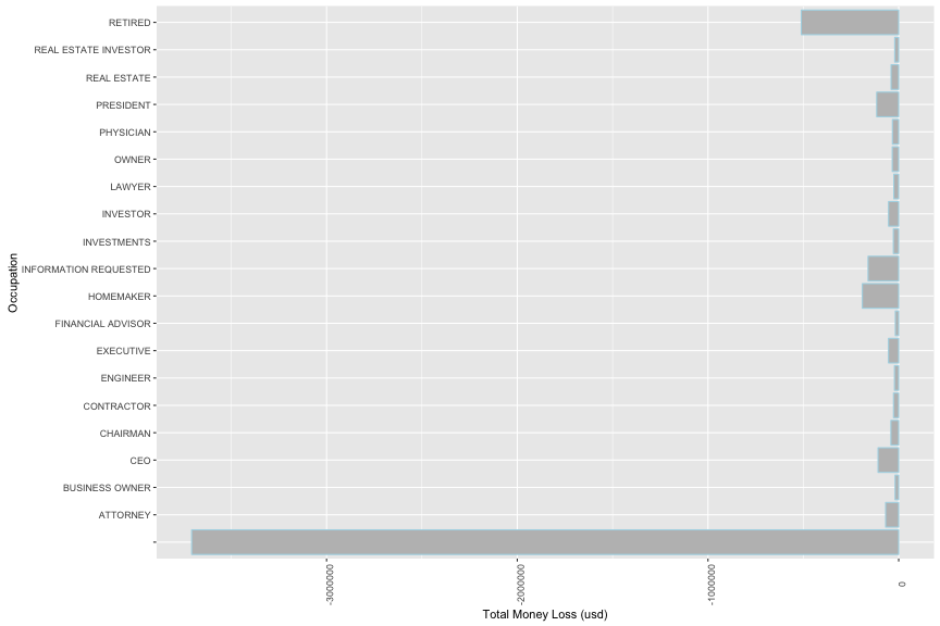
3.4c. Financial Support vs Occupation
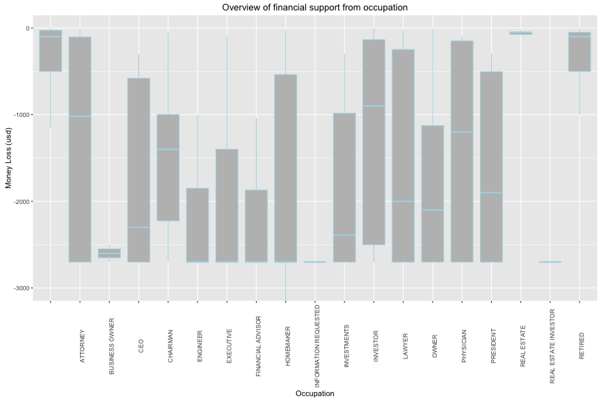
## target_pf_nega$occupation:
##       Min.    1st Qu.     Median       Mean    3rd Qu.       Max.
## -10500.000   -500.000   -100.000   -565.349    -27.000     -0.440
## --------------------------------------------------------
## target_pf_nega$occupation: ATTORNEY
##      Min.   1st Qu.    Median      Mean   3rd Qu.      Max.
## -2700.000 -2700.000 -1020.000 -1414.171  -104.125   -11.450
## --------------------------------------------------------
## target_pf_nega$occupation: BUSINESS OWNER
##    Min. 1st Qu.  Median    Mean 3rd Qu.    Max.
##   -2700   -2650   -2600   -2600   -2550   -2500
## --------------------------------------------------------
## target_pf_nega$occupation: CEO
##     Min.  1st Qu.   Median     Mean  3rd Qu.     Max.
## -2700.00 -2700.00 -2300.00 -1806.25  -580.00  -300.00
## --------------------------------------------------------
## target_pf_nega$occupation: CHAIRMAN
##    Min. 1st Qu.  Median    Mean 3rd Qu.    Max.
##   -2700   -2225   -1400   -1465   -1000     -50
## --------------------------------------------------------
## target_pf_nega$occupation: ENGINEER
##      Min.   1st Qu.    Median      Mean   3rd Qu.      Max.
## -2700.000 -2700.000 -2700.000 -2133.333 -1850.000 -1000.000
## --------------------------------------------------------
## target_pf_nega$occupation: EXECUTIVE
##      Min.   1st Qu.    Median      Mean   3rd Qu.      Max.
## -2700.000 -2700.000 -2700.000 -1957.071 -1399.750  -100.000
## --------------------------------------------------------
## target_pf_nega$occupation: FINANCIAL ADVISOR
##      Min.   1st Qu.    Median      Mean   3rd Qu.      Max.
## -2700.000 -2700.000 -2700.000 -2146.667 -1870.000 -1040.000
## --------------------------------------------------------
## target_pf_nega$occupation: HOMEMAKER
##    Min. 1st Qu.  Median    Mean 3rd Qu.    Max.
## -5400.0 -2700.0 -2700.0 -1835.0  -537.5   -30.0
## --------------------------------------------------------
## target_pf_nega$occupation: INFORMATION REQUESTED
##      Min.   1st Qu.    Median      Mean   3rd Qu.      Max.
## -5400.000 -2700.000 -2700.000 -2462.647 -2700.000  -165.000
## --------------------------------------------------------
## target_pf_nega$occupation: INVESTMENTS
##    Min. 1st Qu.  Median    Mean 3rd Qu.    Max.
##   -2700   -2700   -2390   -1850    -985    -300
## --------------------------------------------------------
## target_pf_nega$occupation: INVESTOR
##      Min.   1st Qu.    Median      Mean   3rd Qu.      Max.
## -2700.000 -2500.000  -900.000 -1159.833  -135.375    -0.240
## --------------------------------------------------------
## target_pf_nega$occupation: LAWYER
##      Min.   1st Qu.    Median      Mean   3rd Qu.      Max.
## -2700.000 -2700.000 -2000.000 -1408.711  -248.400   -30.000
## --------------------------------------------------------
## target_pf_nega$occupation: OWNER
##    Min. 1st Qu.  Median    Mean 3rd Qu.    Max.
## -2700.0 -2700.0 -2100.0 -1727.5 -1127.5   -10.0
## --------------------------------------------------------
## target_pf_nega$occupation: PHYSICIAN
##      Min.   1st Qu.    Median      Mean   3rd Qu.      Max.
## -2700.000 -2700.000 -1200.000 -1385.714  -150.000  -100.000
## --------------------------------------------------------
## target_pf_nega$occupation: PRESIDENT
##      Min.   1st Qu.    Median      Mean   3rd Qu.      Max.
## -2700.000 -2700.000 -1900.000 -1647.857  -505.000  -300.000
## --------------------------------------------------------
## target_pf_nega$occupation: REAL ESTATE
##       Min.    1st Qu.     Median       Mean    3rd Qu.       Max.
## -2700.0000   -75.0000   -50.0000  -411.8983   -50.0000    -7.0000
## --------------------------------------------------------
## target_pf_nega$occupation: REAL ESTATE INVESTOR
##    Min. 1st Qu.  Median    Mean 3rd Qu.    Max.
##   -2700   -2700   -2700   -2700   -2700   -2700
## --------------------------------------------------------
## target_pf_nega$occupation: RETIRED
##      Min.   1st Qu.    Median      Mean   3rd Qu.      Max.
## -5400.000  -500.000  -100.000  -645.571   -50.000    -1.000
The financial support is mostly reduced from people who has unknow occupation (median = 100, max = -10,500)
3.4d. Cross Correlation between features of interest
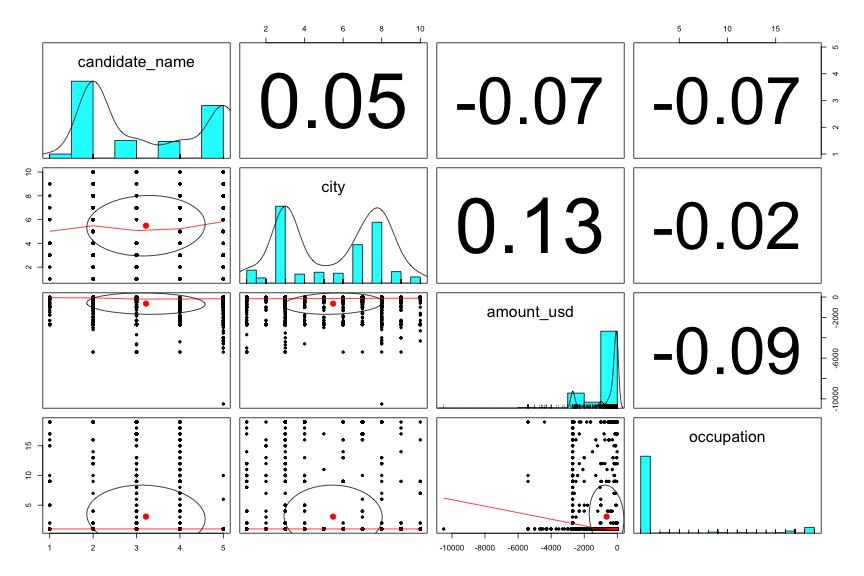
Similar to postive support exploration, I have very low correlation between features of interest.
4. Bivariate Analysis
Talk about some of the relationships you observed in this part of the investigation. How did the feature(s) of interest vary with other features in the dataset?
There is a high correlation between the number of contribution and the amount of money. Hence, a candidate needs to focus on gaining more contribution if he(she) want to increase his(her) election finance. In contrast, there is a risk of losing money when the number of contribution is also correlated to the amount of money loss. This pattern applies to candidate, cities and occupations.
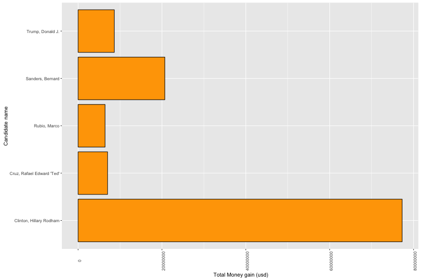
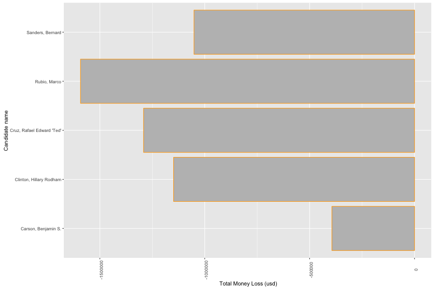
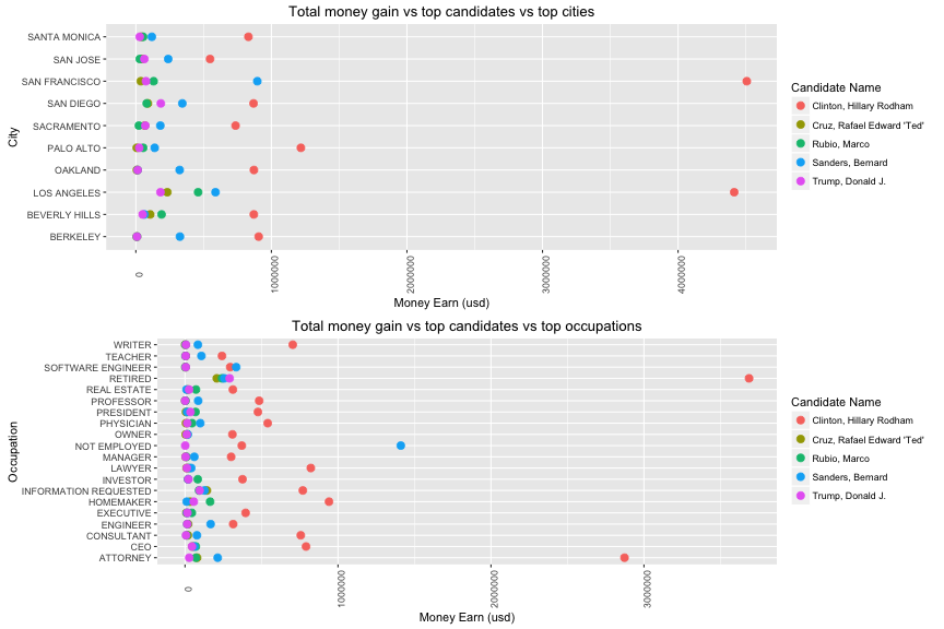
Hilary Clinton is the one who earned biggest money in CA comparing to other candidates with ~ 80 millions and Marco Rubio is the one who lost biggest money in CA with ~ 1,5 millions.
In location, the financial support also depends on the size of city. It is clearly that the two biggest cities in CA have the highest amount of money for this American Election.
In occupation, the interesting point is that retire people contribute much money for American Election 2016. The variance of other features of interest hardly used to predict the financial contribution.
Did you observe any interesting relationships between the other features (not the main feature(s) of interest)?
There is no relationship between other features. It strongly depends on the trust of contributors during the election.
What was the strongest relationship you found?
The strongest relationship that can be found in my exploration is that the magnitude of financial support is strongly correlated with the number of contribution. It doesnot correlated with the social status or location of contributors.
5. Multivariate Plots Section
I applied the same approach as Extra Exploration by create two subset from raw data with following criteria:
-
In top 5 candidate.
-
In top 10 cities.
-
In top 20 occupation.
5.1. Positive Contribution
5.1a. Location
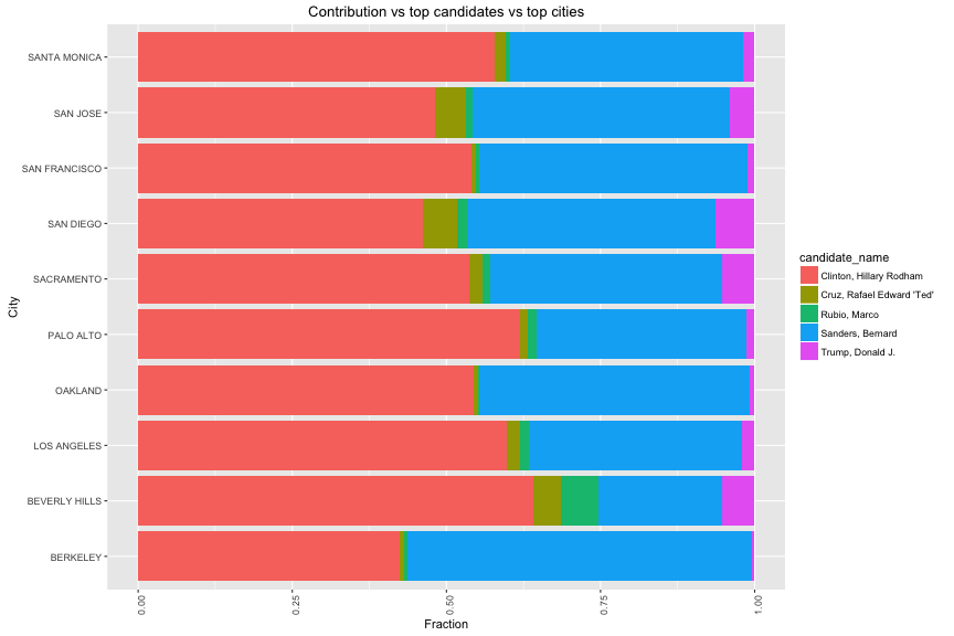
Hilary Clinton received more than 50% of support from 9 of 10 cities except Berkeley. People of Berkerly prefer Bernard Sanders.
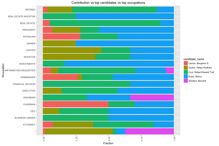
5.1b. Occupation
Let take a look to the faction distribution for each candidate in top 20 jobs.
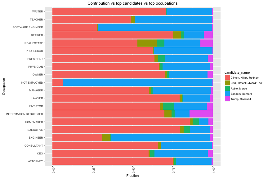
17 of 20 occupation have more than 50% of financial support to Hilary Clinton. Only NOT EMPLOYED and SOFTWARE ENGINEER have more than 50% of their support to Bernard Sanders. Top 1 contributor, retire people also voted for Hilary Clinton.

The graph above shows the number of contribution of each occupation in each cities. In all of occupation, Los Angeles is the city which has biggest number of contribution from retire people. The second place is from retire people in San Francisco.
5.2. Negative Contribution
5.2a. Location
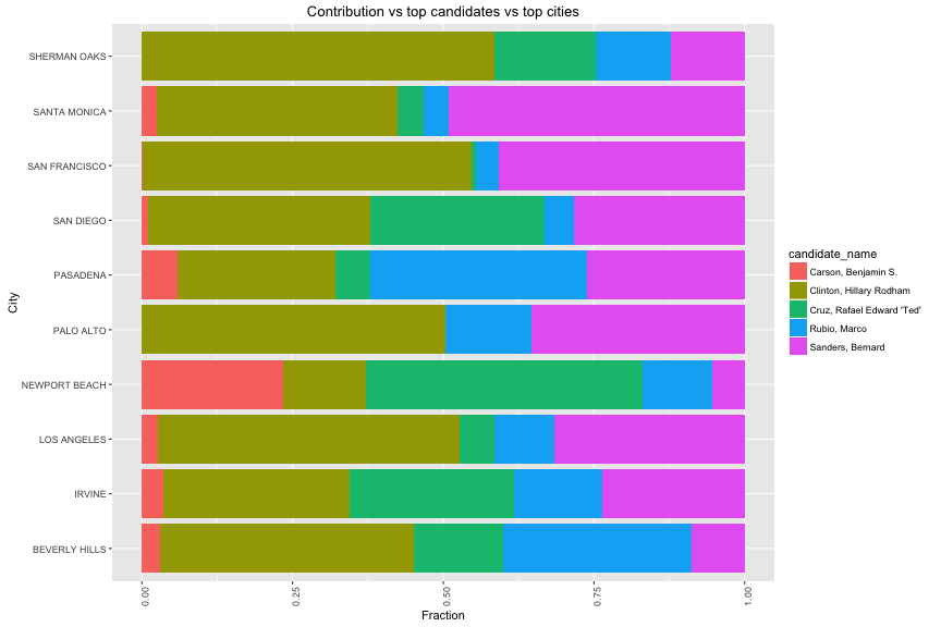
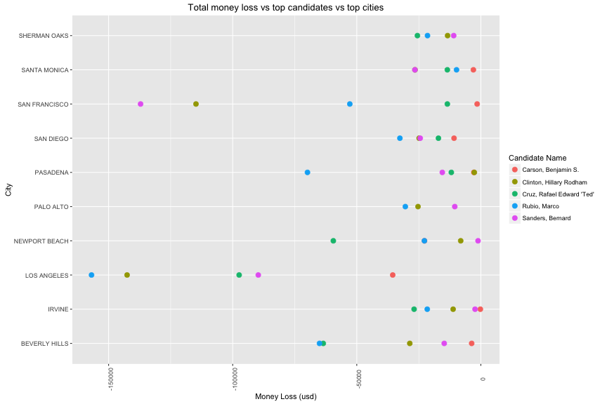
Hilary Clinton (top 1 in positive contribution) received more than 50% of negative contribution in Oakland and San Francisco. Moreover, Marco Rubio is the one who lost biggest money in two largest cities: Los Angeles and San Francisco (6000 usd and 2000 usd respectively).
5.2b. Occupation
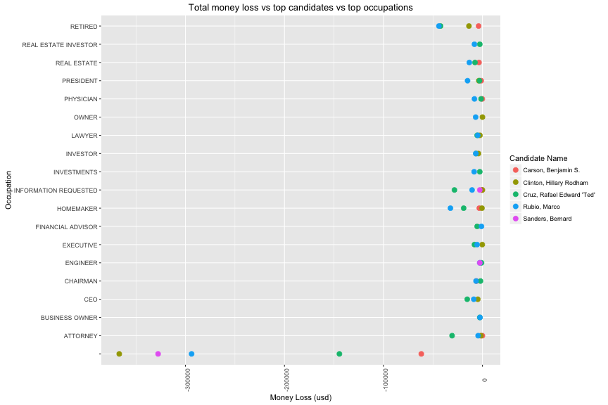
Obviously, Marco Rubio is the one who received the most number of negative contribution from top 20 opccupations. In group of unknow occupation, Hilary Clinton lost biggest money with ~ 400,000 usd.
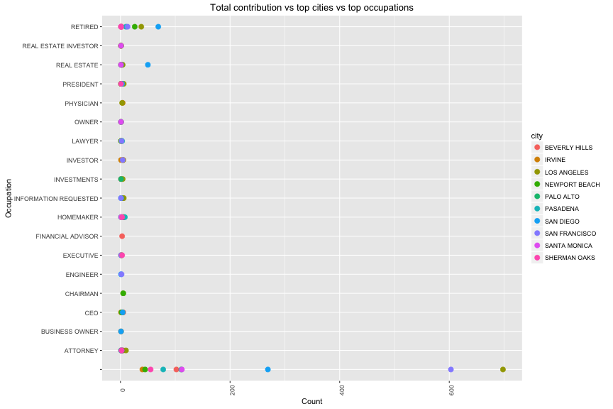
In all of occupation, Los Angeles is the city which has biggest number of negative contribution from unknown people. The second place is from unknown people in San Francisco.
6. Multivariate Analysis
Talk about some of the relationships you observed in this part of the investigation. Were there features that strengthened each other in terms of looking at your feature(s) of interest?
The relationship in this part stated that the candidate who has large number of contribution, will have large financial support (ex: Hilary Clinton). This principle applied to other feature like location (cities) and social status (occupation).
Hilary Clinton won in getting financial support from all of top 10 cities in CA as well as top 20 occupation. The negative finance is varied and depends on candidate name in difference location and occupation.
Were there any interesting or surprising interactions between features?
I didnot see any suprising interactions between features because the number of contribution is the decisive factor to quantify those features of interest and the financial support is strongly related to this number.
7. Final Plots and Summary
Plot one

##     Min.  1st Qu.   Median     Mean  3rd Qu.     Max.
##     0.01    15.00    27.00   130.50    96.50 10800.00
Description one
The distribution of contribution per candidate is very skewed in California. The most favourite candidates are Hilary Clinton and Bernard Sanders with financial contribution > 400,000. Their contributions are 8 times larger than the rest. Additionally, it provides a good starting view to determine candidate’s finance in this state. The amount of contribution is very diversed. Its range mainly from 15 to 96 usd.
Plot two
Description Two
This is the most important plot when I easily observe the trending of financial support and the number of contribution. Clearly, the increase of contribution is correlated to the increase and decrease of money support for candidate (r > 0.90). In the other words, candidate who has large group of contributors will have high chance to get large money support and also have high risk to lose a considerable money. This relationship can be described in linear regression model. In conclusion, if candidates want to enlarge their Election funding, they need to make their group of contributors larger.
Plot three
Description three
These two plots prove that there is no variables of interest that affect money support beside number of contribution. Large city has large money support. Large group of occupation has large money support. The financial contribution for each candidate varied depend on the number of contribution from each cities and each occupation. It stated that the location or the social status is not a factor for changing money support. The size is the main factor. On the other hand, the interesting point is that no labor group (retired or not employed) contributed more money than labor group in this election. Finally, the building of a preditive model is not a good approach for this dataset.
8. Reflection
This financial contribution dataset contains information of more than 1 million observations across 19 variables in California from 2015 to 2016. In each individual variables, I started to select variable that helps me to answer my curiosity and leads to make observations on plots. At last, I explored the financial supports across the candidate, cities and occupation.
I encountered to the positive and negative number in financial report. If I didnot clean them, it would provide incorrect summary of financial support. Hence, I divided this dataset into two subset and did exploration. Moreover, I have categorical variables with more than 1000 factors. My solution is to limit those observations in top 5 candidates who have largest number of contributions in top 20 occupations and in top 10 cities.
There is a strong correlation between the number of contribution and the amount of money (both negative and positive side). There is no correlation between other categorical variables such as candidates, cities, occupations that I am interested. I struggled finding the relation between financial suports and other variables but this mystery is clearer when I realized that other variables are independent factors. So the relation is zero. In this exploration, I would like to provide the influence of candidates to cities and occupations by using the financial contribution. From that, we can estimate the chance of winner among those candidates during this American Election. Where is their strongest location ? Which people believe in their lead ? All those question can be answered by my plots.
However, my exploration has also limitations. Firstly, there is a duplication of money transactions from one unique contributor. Those contributors put money in and out of candidate funding by multiple times. Those activity makes outliers for the analysis and we get incorrect financial support for candidate per contributor. The good solution is making the financial summary of a unique contributor for every candidate. Because of lacking personal information (ex: date of birth, gender), I can not clean these errors correctly. Secondly, there is a group of unknow occupation. This is the intentional bias in which the contributors want to hide their info. This is one obstruction to clean this dataset. Thirdly, I only picked one state of America, it will underestimate the financial support of American Election. In further investigation, I prefer to use larger dataset including other states. Finally, I am not successful in making a predictive model based on categorical variables. That is the next thing I will do soon. The American Election 2016 was over so I hope to get a well-defined dataset.